Parallel Algorithms
flox outsources the core GroupBy operation to the vectorized implementations controlled by the
engine kwarg. Applying these implementations on a parallel array type like dask
can be hard. Performance strongly depends on how the groups are distributed amongst the blocks of an array.
flox implements 4 strategies for grouped reductions, each is appropriate for a particular distribution of groups
among the blocks of a dask array.
Tip
By default, flox >= 0.9.0 will use heuristics to choose a method.
Switch between the various strategies by passing method and/or reindex to either flox.groupby_reduce()
or flox.xarray.xarray_reduce(). Your options are:
The most appropriate strategy for your problem will depend on the chunking of your dataset, and the distribution of group labels across those chunks.
Currently these strategies are implemented for dask. We would like to generalize to other parallel array types as appropriate (e.g. Ramba, cubed, arkouda). Please open an issue to discuss if you are interested.
Background
Without flox installed, Xarray’s GroupBy strategy is to find all unique group labels,
index out each group, and then apply the reduction operation. Note that this only works
if we know the group labels (i.e. you cannot use this strategy to group by a dask array),
and is basically an unvectorized slow for-loop over groups.
Schematically, this looks like (colors indicate group labels; separated groups of colors indicate different blocks of an array):

The first step is to extract all members of a group, which involves a lot of communication and is quite expensive (in dataframe terminology, this is a “shuffle”). This is fundamentally why many groupby reductions don’t work well right now with big datasets.
method="map-reduce"
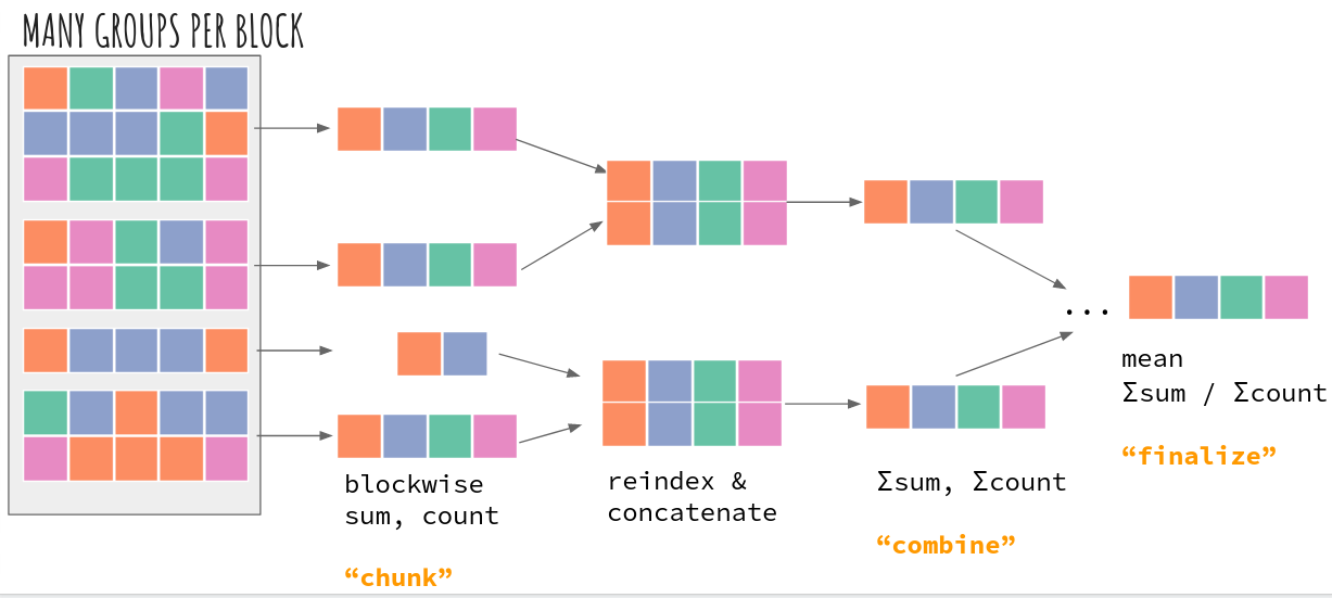
The “map-reduce” strategy is inspired by dask.dataframe.groupby).
The GroupBy reduction is first applied blockwise. Those intermediate results are
combined by concatenating to form a new array which is then reduced
again. The combining of intermediate results uses dask’s _tree_reduce
till all group results are in one block. At that point the result is
“finalized” and returned to the user.
General Tradeoffs
This approach works well when either the initial blockwise reduction is effective, or if the reduction at the first combine step is effective. Here “effective” means we have multiple members of a single group in a block so the blockwise application of groupby-reduce actually reduces values and releases some memory.
One downside is that the final result will only have one chunk along the new group axis.
We have two choices for how to construct the intermediate arrays. See below.
reindex=True
If we know all the group labels, we can do so right at the blockwise step (reindex=True). This matches dask.array.histogram and
xhistogram, where the bin edges, or group labels oof the output, are known. The downside is the potential of large memory use
if number of output groups is much larger than number of groups in a block.

reindex=False
We can reindex at the combine stage to groups present in the blocks being combined (reindex=False). This can limit memory use at the cost
of a performance reduction due to extra copies of the intermediate data during reindexing.

This approach allows grouping by a dask array so group labels can be discovered at compute time, similar to dask.dataframe.groupby.
reindexing to a sparse array
For large numbers of groups, we might be reducing to a very sparse array (e.g. this issue).
To control memory, we can instruct flox to reindex the intermediate results to a sparse.COO array using:
from flox import ReindexArrayType, ReindexStrategy

ReindexStrategy(
    # do not reindex to the full output grid at the blockwise aggregation stage
    blockwise=False,
    # when combining intermediate results after blockwise aggregation, reindex to the
    # common grid using a sparse.COO array type
    array_type=ReindexArrayType.SPARSE_COO,
)
See this user story for more discussion.
Example
For example, consider groupby("time.month") with monthly frequency data and chunksize of 4 along time.
 With
With reindex=True, each block will become 3x its original size at the blockwise step: input blocks have 4 timesteps while output block
has a value for all 12 months. One could use reindex=False to control memory usage but also see method="cohorts" below.
method="blockwise"
One case where method="map-reduce" doesn’t work well is the case of “resampling” reductions. An
example here is resampling from daily frequency to monthly frequency data: da.resample(time="ME").mean()
For resampling type reductions,
Group members occur sequentially (all days in January 2001 occur one after the other)
All groups not of exactly equal length (31 days in January but 28 in most Februaries)
All members in a group are next to each other (if the time series is sorted, which it usually is).
Because there can be a large number of groups, concatenating results for all groups in a single chunk could be catastrophic.
In this case, it makes sense to use dask.dataframe resample strategy which is to rechunk using flox.rechunk_for_blockwise()
so that all members of a group are in a single block. Then, the groupby operation can be applied blockwise.

Tradeoffs
Only works for certain groupings.
Group labels must be known at graph construction time, so this only works for numpy arrays
Currently the rechunking is only implemented for 1D arrays (being motivated by time resampling), but a nD generalization seems possible.
Only can use the
blockwisestrategy for grouping bynDarrays.Works better when multiple groups are already in a single block; so that the initial rechunking only involves a small amount of communication.
method="cohorts"
The map-reduce strategy is quite effective but can involve some unnecessary communication. It can be possible to exploit
patterns in how group labels are distributed across chunks (similar to method="blockwise" above). Two cases are illustrative:
Groups labels can be approximately-periodic: e.g.
time.dayofyear(period 365 or 366) ortime.month(period 12). Consider our earlier example,groupby("time.month")with monthly frequency data and chunksize of 4 alongtime.
Because a chunksize of 4 evenly divides the number of groups (12) all we need to do is index out blocks
0, 3, 7 and then apply the "map-reduce"strategy to form the final result for months Jan-Apr. Repeat for the remaining groups of months (May-Aug; Sep-Dec) and then concatenate.Groups can be spatially localized like the blockwise case above, for example grouping by country administrative boundaries like counties or districts. In this case, concatenating the result for the northwesternmost county or district and the southeasternmost district can involve a lot of wasteful communication (again depending on chunking).
For such cases, we can adapt xarray’s shuffling or subsetting strategy by indexing out “cohorts” or group labels that tend to occur next to each other.
A motivating example : time grouping
One example is the construction of “climatologies” which is a climate science term for something like groupby("time.month")
(“monthly climatology”) or groupby("time.dayofyear") (“daily climatology”). In these cases,
Groups occur sequentially (day 2 is always after day 1; and February is always after January)
Groups are approximately periodic (some years have 365 days and others have 366)
Consider our earlier example, groupby("time.month") with monthly frequency data and chunksize of 4 along time.
With method="map-reduce", reindex=True, each block will become 3x its original size at the blockwise step: input blocks have 4 timesteps while output block
has a value for all 12 months. Note that the blockwise groupby-reduction does not reduce the data since there is only one element in each
group. In addition, since map-reduce will make the final result have only one chunk of size 12 along the new month
dimension, the final result has chunk sizes 3x that of the input, which may not be ideal.
However, because a chunksize of 4 evenly divides the number of groups (12) all we need to do is index out blocks
0, 3, 7 and then apply the "map-reduce" strategy to form the final result for months Jan-Apr. Repeat for the
remaining groups of months (May-Aug; Sep-Dec) and then concatenate. This is the essence of method="cohorts"
Summary
We can generalize this idea for more complicated problems (inspired by the split_outkwarg in dask.dataframe.groupby)
We first apply the groupby-reduction blockwise, then split and reindex blocks to create a new array with which we complete the reduction
using map-reduce. Because the split or shuffle step occurs after the blockwise reduction, we sometimes communicate a significantly smaller
amount of data than if we split or shuffled the input array.

Tradeoffs
Group labels must be known at graph construction time, so this only works for numpy arrays.
This does require more tasks and a more complicated graph, but the communication overhead can be significantly lower.
The detection of “cohorts” is currently slow but could be improved.
The extra effort of detecting cohorts and multiple copying of intermediate blocks may be worthwhile only if the chunk sizes are small relative to the approximate period of group labels, or small relative to the size of spatially localized groups.
Example : sensitivity to chunking
One annoyance is that if the chunksize doesn’t evenly divide the number of groups, we still end up splitting a number of chunks.
Consider our earlier example, groupby("time.month") with monthly frequency data and chunksize of 4 along time.
flox can find these cohorts, below it identifies the cohorts with labels 1,2,3,4; 5,6,7,8, and 9,10,11,12.
preferred_method, chunks_cohorts = flox.core.find_group_cohorts(labels, chunks)
chunks_cohorts.values()
dict_values([[0, 1, 2, 3], [4, 5, 6, 7], [8, 9, 10, 11]])
Now consider chunksize=5.

dict_values([[0, 10, 11], [1], [2, 3], [4, 5], [6, 7], [8, 9]])
We find 7 cohorts (note the original xarray strategy is equivalent to constructing 12 cohorts).
In this case, it seems to better to rechunk to a size of 4 (or 6) along time.
Indeed flox’s heuristics think "map-reduce" is better for this case:
preferred_method
'map-reduce'
Example : spatial grouping
Spatial groupings are particularly interesting for the "cohorts" strategy. Consider the problem of computing county-level
aggregated statistics (example blog post). There are ~3100 groups (counties), each marked by
a different color. There are ~2300 chunks of size (350, 350) in (lat, lon). Many groups are contained to a small number of chunks:
see left panel where the grid lines mark chunk boundaries.
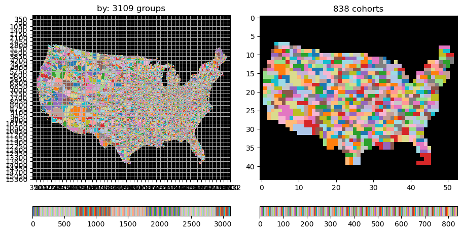
This seems like a good fit for 'cohorts': to get the answer for a county in the Northwest US, we needn’t look at values
for the southwest US. How do we decide that automatically for the user?
Heuristics
flox >=0.9 will automatically choose method for you. To do so, we need to detect how each group
label is distributed across the chunks of the array; and the degree to which the chunk distribution for a particular
label overlaps with all other labels. The algorithm is as follows.
First determine which labels are present in each chunk. The distribution of labels across chunks is represented internally as a 2D boolean sparse array
S[chunks, labels].S[i, j] = 1when labeljis present in chunki.Then we look for patterns in
Sto decide if we can use"blockwise". The dark color cells are1at that cell inS.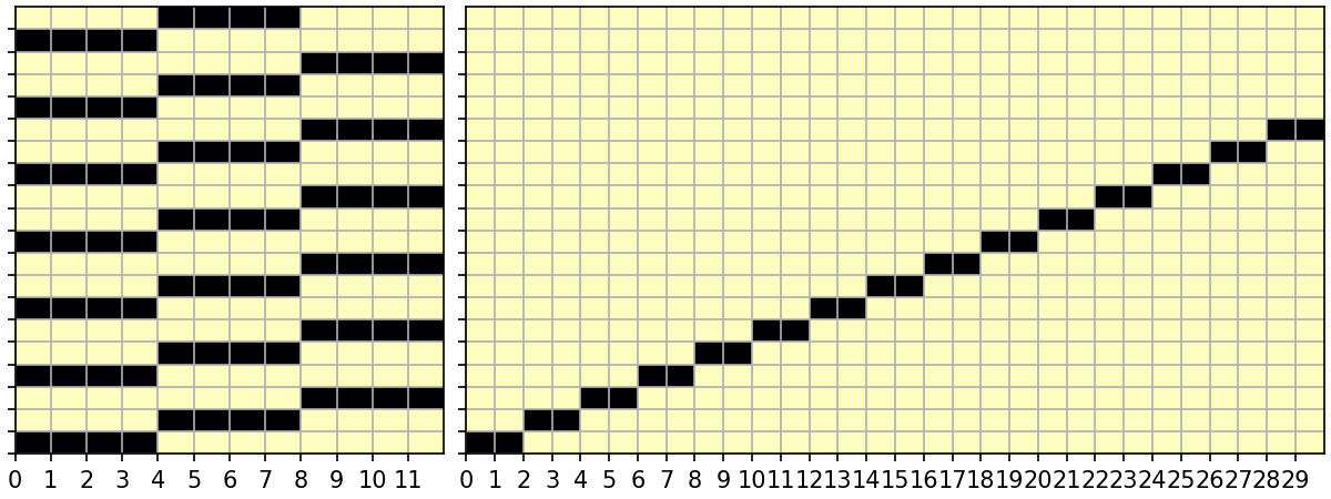
On the left, is a monthly grouping for a monthly time series with chunk size 4. There are 3 non-overlapping cohorts so
method="cohorts"is perfect.On the right, is a resampling problem of a daily time series with chunk size 10 to 5-daily frequency. Two 5-day periods are exactly contained in one chunk, so
method="blockwise"is perfect.
The metric used for determining the degree of overlap between the chunks occupied by different labels is containment. For each label
iwe can quickly compute containment against all other labelsjasC = S.T @ S / number_chunks_per_label. Here isCfor a range of chunk sizes from 1 to 12, for computing the monthly mean of a monthly time series problem, [the title on each image is(chunk size, sparsity)].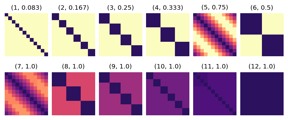
To choose between
"map-reduce"and"cohorts", we need a summary measure of the degree to which the labels overlap with each other. We can use sparsity — the number of non-zero elements inCdivided by the number of elements inC,C.nnz/C.size. We use sparsity(S) as an approximation for the sparsity(C) to avoid a potentially expensive sparse matrix dot product whenSisn’t particularly sparse. When sparsity(S) > 0.4 (arbitrary), we choose"map-reduce"since there is decent overlap between (any) cohorts. Otherwise we use"cohorts".
Cool, isn’t it?!
For reference here is S and C for the US county groupby problem:
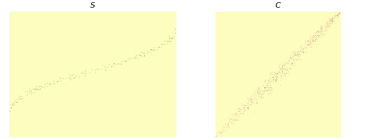 The sparsity of
 C is 0.006, so "cohorts" seems a good strategy here.